Encoder-only Transformer model Fine-tuning을 통해 CoLA 데이터셋 분류하기 & Scheduler-Free 적용하기

Pretraining BERT model with Code example & using The Road Less Scheduled
1. Introduction
나에게 주어진 Task는 다음과 같다.
- (Assignment 1) 주어진 영어 문장에 대해 문법 적합성 판정을 이진분류(binary classification)하는 데이터셋인 The Corpus of Linguistic Acceptability (CoLA) dataset 위에서 Transformer(Encoder-only) 모델을 파인튜닝하여 언어 모델의 문법 적합성 분류 성능을 올리는 것.
2. Assignment 1
우선 CoLA dataset을 로드한다.
1
2
3
4
5
6
7
8
9
10
import pandas as pd
# Load the dataset into a pandas dataframe.
df = pd.read_csv("./cola_public/raw/in_domain_train.tsv", delimiter='\t', header=None, names=['sentence_source', 'label', 'label_notes', 'sentence'])
# Report the number of sentences.
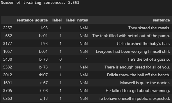
print('Number of training sentences: {:,}\n'.format(df.shape[0]))
# Display 10 random rows from the data.
df.sample(10)
위 코드의 출력 결과는 다음과 같다.
트랜스포머 모델을 학습하기 위해 우리가 건드릴 수 있는 파라미터로는 주로 Learning rate, Batch size, Max epochs가 있다.
그리고 Encoder-only 언어모델 중 하나를 선택해 어떤 모델을 이용할 지 판단할 수 있다. Encoder-only 모델에는 대표적으로 2017년에 구글에서 발표한 BERT(Bidirection Encoder Representations from Transformer)가 있다.
내가 이번 태스크에서 사용한 모델은 BERT를 기반으로 하여 BERT에서 파생된 모델인 ‘roBERTa’, ‘ERNIE-2.0’, ‘Albert’, ‘xlNET’, ‘Electra’ 를 동일한 파라미터 값(Learning Rate : 1e-5, Batch size=32, Epochs=10)을 통하여 비교하였다.
이를 통하여 가장 성능이 좋은 모델을 고정하여 나머지 파라미터를 조절하기로 하였다.
모델을 선언하여, 해당 모델에서 쓰이는 토크나이저(tokenizer)를 호출하여야 한다. 토크나이저를 호출하는 코드는 다음과 같다.
1
2
3
4
5
6
7
8
9
10
from transformers import AutoTokenizer

# Load the BERT tokenizer.
print('Loading BERT tokenizer...')
tokenizer = AutoTokenizer.from_pretrained(pretrained_model, do_lower_case=True) #do_lower_case : 소문자로 치환
'''
Original:  Our friends won't buy this analysis, let alone the next one we propose.
Tokenized:  ['our', 'friends', 'won', "'", 't', 'buy', 'this', 'analysis', ',', 'let', 'alone', 'the', 'next', 'one', 'we', 'propose', '.']
Token IDs:  [2256, 2814, 2180, 1005, 1056, 4965, 2023, 4106, 1010, 2292, 2894, 1996, 2279, 2028, 2057, 16599, 1012]
'''
Original 문자가 ‘Our friends won’t buy this analysis, let alone the next one we propose.’ 일 경우,
이를 tokenize한 결과는 [‘our’, ‘friends’, ‘won’, “’”, ‘t’, ‘buy’, ‘this’, ‘analysis’, ‘,’, ‘let’, ‘alone’, ‘the’, ‘next’, ‘one’, ‘we’, ‘propose’, ‘.’] 와 같다.
이렇게 토큰화된 문자들은 임베딩 과정을 거치기 전에, Token ID 사전과 일대일 매칭이 되어있는 Token ID(number)로 변환된다.
우리는 CoLA dataset을 tokenize하고, token id들을 생성해야 한다. 그 코드는 아래와 같다.
1
2
3
4
5
6
7
8
9
10
11
12
13
14
15
16
17
18
19
20
21
22
23
24
25
26
27
28
29
30
31
32
33
34
35
36
37
38
39
40
41
42
43
44
45
46
47
48
49
max_len = 0

# For every sentence...
for sent in sentences:
    # Tokenize the text and add `[CLS]` and `[SEP]` tokens.
    input_ids = tokenizer.encode(sent, add_special_tokens=True)

    # Update the maximum sentence length.
    max_len = max(max_len, len(input_ids))

print('Max sentence length: ', max_len)

import torch
# Tokenize all of the sentences and map the tokens to thier word IDs.
input_ids = []
attention_masks = []

# For every sentence...
for sent in sentences:
    # `encode_plus` will:
    #   (1) Tokenize the sentence.
    #   (2) Prepend the `[CLS]` token to the start.
    #   (3) Append the `[SEP]` token to the end.
    #   (4) Map tokens to their IDs.
    #   (5) Pad or truncate the sentence to `max_length`
    #   (6) Create attention masks for [PAD] tokens.
    encoded_dict = tokenizer.encode_plus(
                        sent,                      # Sentence to encode.
                        add_special_tokens = True, # Add '[CLS]' and '[SEP]'
                        max_length = 64,           # Pad & truncate all sentences.
                         pad_to_max_length = True,
                        return_attention_mask = True,   # Construct attn. masks.
                        return_tensors = 'pt',     # Return pytorch tensors.
                   )

    # Add the encoded sentence to the list.
    input_ids.append(encoded_dict['input_ids'])

    # And its attention mask (simply differentiates padding from non-padding).
    attention_masks.append(encoded_dict['attention_mask'])

# Convert the lists into tensors.
input_ids = torch.cat(input_ids, dim=0)
attention_masks = torch.cat(attention_masks, dim=0)
labels = torch.tensor(labels)

# Print sentence 0, now as a list of IDs.
print('Original: ', sentences[0])
print('Token IDs:', input_ids[0])
여기서 언어모델에 필요한 special token이 들어간다.
BERT 계열 모델에서는 [CLS] 토큰과 [SEP] 토큰이 special token으로 존재한다.
[CLS] 토큰은 모델에 입력되는 문장의 시작임을 알려주고, [SEP] 토큰은 입력되는 문장이 끝났음을 알려준다.
Tokenize한 데이터를
- Train-Test-Valid Split을 진행하고, Dataloader 선언자로 변환
- Transformer 모델 선언, 최적화를 위한 Optimizer 선언(AdamW), 학습률 스케줄러인 Learning Rate Scheluder 선언(linear scheduler)
- 마지막으로 Tranformer 언어모델 훈련을 진행한다.
이 단계들의 코드는 아래와 같다.
Train-Test Split
1
2
3
4
5
6
7
8
9
10
11
12
13
14
15
16
17
18
from torch.utils.data import TensorDataset, random_split

# Combine the training inputs into a TensorDataset.
dataset = TensorDataset(input_ids, attention_masks, labels)

# Create a 80-10-10 train-validation-test split.

# Calculate the number of samples to include in each set.
train_size = int(0.8 * len(dataset))
val_size = int(0.1 * len(dataset))
test_size = len(dataset) - train_size - val_size

# Divide the dataset by randomly selecting samples.
train_dataset, val_dataset, test_dataset = random_split(dataset, [train_size, val_size, test_size], generator=torch.Generator().manual_seed(42))

print('{:>5,} training samples'.format(train_size))
print('{:>5,} validation samples'.format(val_size))
print('{:>5,} test samples'.format(test_size))
1
2
3
4
5
6
7
8
9
10
11
12
13
14
15
16
17
18
19
20
21
22
from torch.utils.data import DataLoader, RandomSampler, SequentialSampler

def ret_dataloader():
    print('batch_size = ', batch_size)
    train_dataloader = DataLoader(
                train_dataset,  # The training samples.
                sampler = RandomSampler(train_dataset), # Select batches randomly
                batch_size = batch_size # Trains with this batch size.
            )

    validation_dataloader = DataLoader(
                val_dataset, # The validation samples.
                sampler = SequentialSampler(val_dataset), # Pull out batches sequentially.
                batch_size = batch_size # Evaluate with this batch size.
            )

    test_dataloader = DataLoader(
                test_dataset, # The validation samples.
                sampler = SequentialSampler(test_dataset), # Pull out batches sequentially.
                batch_size = batch_size # Evaluate with this batch size.
            )
    return train_dataloader,validation_dataloader,test_dataloader
Load Pre-trained BERT model
1
2
3
4
5
6
7
8
9
10
11
12
13
14
15
16
17
18
19
20
21
22
23
24
25
26
27
28
29
30
31
32
33
34
35
36
37
38
39
40
41
42
43
44
45
46
47
48
49
50
51
52
53
54
55
from transformers import AdamW, AutoModelForSequenceClassification

def ret_model():

    model = AutoModelForSequenceClassification.from_pretrained(
        pretrained_model,
        num_labels = 2,
        output_attentions = False, # Whether the model returns attentions weights.
        output_hidden_states = False, # Whether the model returns all hidden-states.
    )

    return model

def ret_optim(model):
    print('Learning_rate = ', learning_rate)
    optimizer = AdamW(model.parameters(),
                      lr = learning_rate,
                      eps = 1e-8
                    )
    return optimizer

from transformers import get_linear_schedule_with_warmup

def ret_scheduler(train_dataloader,optimizer):

    print('epochs =>', epochs)
    # Total number of training steps is [number of batches] x [number of epochs].
    # (Note that this is not the same as the number of training samples).
    total_steps = len(train_dataloader) * epochs

    # Create the learning rate scheduler.
    scheduler = get_linear_schedule_with_warmup(optimizer,
                                                num_warmup_steps = 0, # Default value in run_glue.py
                                                num_training_steps = total_steps)
    return scheduler

    import numpy as np

# Function to calculate the accuracy of our predictions vs labels
def flat_accuracy(preds, labels):
    pred_flat = np.argmax(preds, axis=1).flatten()
    labels_flat = labels.flatten()
    return np.sum(pred_flat == labels_flat) / len(labels_flat)
import time
import datetime

def format_time(elapsed):
    '''
    Takes a time in seconds and returns a string hh:mm:ss
    '''
    # Round to the nearest second.
    elapsed_rounded = int(round((elapsed)))

    # Format as hh:mm:ss
    return str(datetime.timedelta(seconds=elapsed_rounded))
The Train Function
1
2
3
4
5
6
7
8
9
10
11
12
13
14
15
16
17
18
19
20
21
22
23
24
25
26
27
28
29
30
31
32
33
34
35
36
37
38
39
40
41
42
43
44
45
46
47
48
49
50
51
52
53
54
55
56
57
58
59
60
61
62
63
64
65
66
67
68
69
70
71
72
73
74
75
76
77
78
79
80
81
82
83
84
85
86
87
88
89
90
91
92
93
94
95
96
97
98
99
100
101
102
103
104
105
106
107
108
109
110
111
112
113
114
115
116
117
118
119
120
121
122
123
124
125
126
127
128
129
130
131
132
133
134
135
136
137
138
139
140
141
142
143
144
145
146
147
148
149
150
151
152
153
154
155
156
157
158
159
160
161
162
163
164
165
166
167
168
169
170
171
172
173
174
175
176
177
178
179
180
181
182
183
184
185
186
187
188
189
190
191
192
193
194
import random
import numpy as np
    # Set the seed value all over the place to make this reproducible.
def train():
    device = torch.device('cuda' if torch.cuda.is_available() else 'cpu')
    print(device)
    model = ret_model()
    model.to(device)
    train_dataloader,validation_dataloader,test_dataloader = ret_dataloader()
    optimizer = ret_optim(model)
    scheduler = ret_scheduler(train_dataloader,optimizer)

    seed_val = 42
    best_val_acc = 0

    random.seed(seed_val)
    np.random.seed(seed_val)
    torch.manual_seed(seed_val)
    training_stats = []

    # Measure the total training time for the whole run.
    total_t0 = time.time()
    # For each epoch...
    for epoch_i in range(0, epochs):
        # ========================================
        #               Training
        # ========================================
        # Perform one full pass over the training set.

        print("")
        print('======== Epoch {:} / {:} ========'.format(epoch_i + 1, epochs))
        print('Training...')

        # Measure how long the training epoch takes.
        t0 = time.time()

        # Reset the total loss for this epoch.
        total_train_loss = 0

        # Put the model into training mode. Don't be mislead--the call to `train` just changes the *mode*, it doesn't *perform* the training.
        model.train()

        # For each batch of training data...
        for step, batch in enumerate(train_dataloader):

            # Progress update every 40 batches.
            if step % 40 == 0 and not step == 0:
                # Calculate elapsed time in minutes.
                elapsed = format_time(time.time() - t0)
                # Report progress.
                print('  Batch {:>5,}  of  {:>5,}.    Elapsed: {:}.'.format(step, len(train_dataloader), elapsed))

            # Unpack this training batch from our dataloader.
            # As we unpack the batch, we'll also copy each tensor to the GPU using the`to` method.
            # `batch` contains three pytorch tensors:
            b_input_ids = batch[0].to(device)  #   [0]: input ids
            b_input_mask = batch[1].to(device) #   [1]: attention masks
            b_labels = batch[2].to(device)     #   [2]: labels

            model.zero_grad()
            (output) = model(b_input_ids,
                                token_type_ids=None,
                                attention_mask=b_input_mask,
                                labels=b_labels)
            loss = output[0]
            logits = output[1]
            # Accumulate the training loss over all of the batches so that we can calculate the average loss at the end.
            total_train_loss += loss.item()

            # Perform a backward pass to calculate the gradients.
            loss.backward()

            # Clip the norm of the gradients to 1.0.
            # This is to help prevent the "exploding gradients" problem.
            torch.nn.utils.clip_grad_norm_(model.parameters(), 1.0)

            # Update parameters and take a step using the computed gradient.
            # The optimizer dictates the "update rule"--how the parameters are
            # modified based on their gradients, the learning rate, etc.
            optimizer.step()

            # Update the learning rate.
            scheduler.step()

        # Calculate the average loss over all of the batches.
        avg_train_loss = total_train_loss / len(train_dataloader)

        # Measure how long this epoch took.
        training_time = format_time(time.time() - t0)

        print("")
        print("  Average training loss: {0:.2f}".format(avg_train_loss))
        print("  Training epcoh took: {:}".format(training_time))

        # ========================================
        #               Validation
        # ========================================
        print("")
        print("Running Validation...")
        t0 = time.time()

        # Put the model in evaluation mode--the dropout layers behave differently during evaluation.
        model.eval()

        # Tracking variables
        total_eval_accuracy = 0
        total_eval_loss = 0
        nb_eval_steps = 0

        # Evaluate data for one epoch
        for batch in validation_dataloader:
            b_input_ids = batch[0].cuda()       #   [0]: input ids
            b_input_mask = batch[1].to(device)  #   [1]: attention masks
            b_labels = batch[2].to(device)      #   [2]: labels

            with torch.no_grad():
                output = model(b_input_ids,
                                      token_type_ids=None,
                                      attention_mask=b_input_mask,
                                      labels=b_labels)
                loss = output[0]
                logits = output[1]

            total_eval_loss += loss.item()
            logits = logits.detach().cpu().numpy()
            label_ids = b_labels.to('cpu').numpy()
            total_eval_accuracy += flat_accuracy(logits, label_ids)

        # Report the final accuracy for this validation run.
        avg_val_accuracy = total_eval_accuracy / len(validation_dataloader)
        print("  Accuracy: {0:.2f}".format(avg_val_accuracy))

        # Calculate the average loss over all of the batches.
        avg_val_loss = total_eval_loss / len(validation_dataloader)

        # Measure how long the validation run took.
        validation_time = format_time(time.time() - t0)
        print("  Validation Loss: {0:.2f}".format(avg_val_loss))
        print("  Validation took: {:}".format(validation_time))

        if avg_val_accuracy > best_val_acc:
            print("Saving the best model...")
            torch.save({'epoch': epoch_i, 'model_state_dict': model.state_dict(),'optimizer_state_dict': optimizer.state_dict(),'loss': avg_val_loss,},
                       "best_model.pth")
            best_val_acc = avg_val_accuracy

        # Record all statistics from this epoch.
        training_stats.append(
            {
                'epoch': epoch_i + 1,
                'Training Loss': avg_train_loss,
                'Valid. Loss': avg_val_loss,
                'Valid. Accur.': avg_val_accuracy,
                'Training Time': training_time,
                'Validation Time': validation_time
            }
        )

    print("")
    print("Training complete!")

    print("Total training took {:} (h:mm:ss)".format(format_time(time.time()-total_t0)))

    print("Evaluate on Test set!")
    checkpoint = torch.load("best_model.pth")
    model.load_state_dict(checkpoint['model_state_dict'])
    model.eval()
    total_eval_accuracy = 0
    for batch in test_dataloader:
        b_input_ids = batch[0].cuda()
        b_input_mask = batch[1].to(device)
        b_labels = batch[2].to(device)

        with torch.no_grad():
            output = model(b_input_ids,
                                  token_type_ids=None,
                                  attention_mask=b_input_mask,
                                  labels=b_labels)
            loss = output[0]
            logits = output[1]

        total_eval_loss += loss.item()
        logits = logits.detach().cpu().numpy()
        label_ids = b_labels.to('cpu').numpy()
        total_eval_accuracy += flat_accuracy(logits, label_ids)

    avg_test_accuracy = total_eval_accuracy / len(test_dataloader)
    print("Test Accuracy: {0:.4f}".format(avg_test_accuracy))
    print("learning rate: ", learning_rate)
    print("epochs: ", epochs)
    print("batch size: ", batch_size)
    print("model name: ", pretrained_model)
train()
이렇게 모델의 훈련을 진행하고, 훈련된 모델의 최종 Test Accuracy를 산출한다.
그 결과는 다음과 같다.
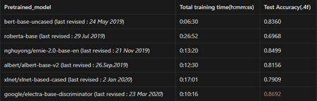
모델의 성능을 비교할 때 쓰이는 지표에는 주로 성능과 학습 시간이 있다. 둘 다 중요하긴 하지만, 태스크의 목표가 분류 성능을 올리는 것이므로 Test Accuracy를 먼저 보았다.
BERT부터 시작하여 model의 paper가 Last revised된 순서대로 pre-training을 진행한 결과, Encoder-only LLM 중에서 늦게 출시된 Google의 Electra가 가장 높은 성능을 보였다.
이에 따라서 Electra를 base model로 두어 나머지 세 개의 파라미터를 조정하면서 실험을 진행하였다.
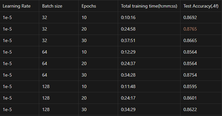
우선 학습률을 고정한 상태에서 Batch size와 Epoch를 조절하여 비교를 진행하였다. 그 결과는 아래의 표와 같다.
일반적으로 딥러닝 모델의 학습에서 input data의 batch size가 작을 경우, sampling되는 표본의 수가 많으므로 noise가 더 많은 gradient update를 진행할 수 있다. 여기서 noise는 data의 불확실성 또는 복잡한 패턴의 변화가 있다. 이로 인해 과적합의 위험이 줄어들어 일반화 성능이 커지는 장점이 있다. 다만 noise가 많으므로 gradient update의 수렴이 어려워질 수 있다.
Input data의 batch size가 클 경우에는 sampling되는 표본의 noise가 줄어들어 gradient update의 수렴 안정성이 증가하지만, 이로 인해 모델이 과적합할 위험이 커진다.
Epoch 또한 batch size와 비슷한 추세를 보인다. Epoch를 크게 하여 여러 번 훈련을 진행할 경우, 모델이 주어진 training dataset에 과적합되어 Valid/Test dataset에 대한 일반화 성능이 낮아질 수 있다.
Epoch가 작을 경우 일반화 성능에 대한 Robustness(강건성)가 증가하지만, 모델의 학습 성능 자체가 열악해질 가능성이 있다.
위의 표에서 고정된 학습률에서 Batch size = [32, 64, 128], Epochs = [10, 20, 30]으로 변인을 두어 실험을 진행하였다.
같은 batch size에서 epochs를 늘릴수록 성능이 높은 경향성(batch size=32 제외)을 보이고, 같은 epochs에서 batch size가 32, 128, 64의 순으로 성능이 높은 경향성을 보였다. 하지만 의외로 최고의 성능은 batch size=32, epochs=20에서 제일 높았다.
일반적으로 딥러닝 모델의 학습률이 높으면 모델의 수렴이 빠르다고 하지만, 너무 높을 경우 오히려 수렴하지 못하고 발산하거나 최적점 근처에서 진동할 가능성이 있다.
반대로 학습률이 낮을 경우 모델이 천천히 수렴하여 학습 시간이 길어질 수 있지만, 더 안정적인 학습이 될 수 있다. 다만 학습률이 너무 낮을 경우 local minima에 갇혀 더 좋은 최적해를 찾지 못할 수도 있다.
적절한 학습률을 찾기 위해 학습률 스케줄러를 이용하기도 한다. 주어진 코드에서는 linear scheduler로 학습률 스케줄링을 진행한 것을 알 수 있다. 학습률 스케줄러는 linear scheduler 외에도 power scheduling, exponential scheduling, piecewise constant scheduling, performance scheduling, 1-cycle scheduling 등이 있다. 모델링 상황에 맞게 적절한 방법을 쓰는 것이 좋다.
Electra의 paper에 따르면, Electra를 제작한 연구진들은 초기 학습률 [1e-4, 2e-4, 3e-4, 5e-4] 중에서 최고의 실험 성능을 도출하였다고 한다.
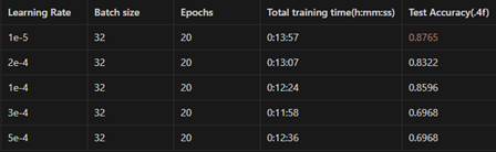
따라서 본 태스크에서 초기에 주어진 학습률인 1e-5 외에 논문에 언급된 네 개의 학습률로 pretraining을 진행하였다. 그 결과는 아래와 같다.
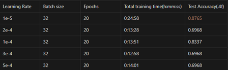
결과를 살펴보면 학습률에 따라 모델 학습 시간에 약간씩 차이가 있지만 심하게 나진 않는다.
성능 면에선 학습률을 1e-4로 두었을 때 제일 높은 성능을 보였다. 그보다 크게 학습률을 설정할 경우 전부 Test Acc가 0.6968로 나온 것으로 보아 수렴하지 못하고 갇힌 것으로 보인다.
같은 batch size, epochs에서 Electra paper에서 언급된 네 개의 학습률보다 처음의 학습률 1e-5의 성능(0.8765)이 젤이 노다. 이 이유는 잘 모르겠다. 학습률과 관련해서 여러 가지 실험을 통해 경향성을 제시한 논문들이 있지만, 이러한 부분의 확실한 인과성을 밝히기 위한 연구가 필요하다고 느낀다.
2024년 5월 24일, FAIR at Meta에서 학습률 스케줄링을 이용하지 않는 최적화 방법에 대한 paper와 github code를 발표하였다. 이 논문에선 학습률 스케줄링을 진행하지 않고 모멘텀 기반의 지수 이동 평균(EMA) 기법을 이용한 파라미터 업데이트를 통해 다양한 최적화 문제에서 뛰어난 성능을 발휘하는 Schedule-Free optimizing을 제안하였다.
Schedule-Free AdamW optimizer를 이용하여 앞에서 진행한 다섯 개의 학습률 pretraining 실험을 진행하였다. 그 결과는 아래와 같다.
Schedule-Free optimizer를 이용한 결과를 분석해보면, linear scheduler를 이용했을 때와 비교하여 초기 학습률 설정에 대해 더 robust함을 알 수 있다. 그 이유를 분석해보자면, schedule-free에선 학습률을 훈련 과정 중에 평균화 기법 이용하여 동적으로 조정하며 momentum을 통해 큰 기울기 변동을 완화하여 더 안정적인 학습을 진행하기 때문이다.
진행한 실험 최종적으로 [Pretrained Model : google/electra, Learning Rate : 1e-5, Batch size : 32, Epochs : 20]의 파라미터로 최적의 성능을 달성하였다.